Introduction
Welcome to a primer on single-cell RNA sequencing (scRNA-seq). Studies suggest that new information is retained more effectively when paired with a high-level overview, this overview act as a sort of cognitive scaffolding for which to build details later on. With that in mind, this primer isn’t a deep-dive tutorial or comprehensive guide. Instead, it aims to provide a high-level framework: what single-cell RNA-seq is, why it’s useful, the core steps of a typical workflow, and some common pitfalls to be aware of.
What Is Single-Cell RNA-Seq?
At its simplest, single-cell RNA-seq involves sequencing mRNA from individual cells by generating cDNA libraries tagged with barcodes that identify both the cell and each molecule sequenced. For the 10x Genomics Chromium platform, these barcodes are typically 16 bp (cell barcode) and 12 bp (unique molecular identifier, or UMI) in length.
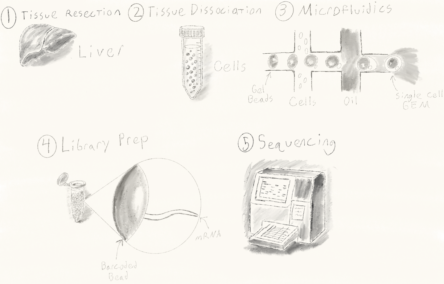
This technology allows us to reconstruct a partial transcriptomic profile per cell, enabling insights into cellular identity, diversity, and state. While it may seem abstract, the basics of the wet-lab workflow help demystify how it works—and why certain analysis pitfalls can occur. Here’s a step-by-step overview (visual learners may find the field sketch below helpful as a guide):
Wet Lab Workflow
-
Tissue Resection A physical tissue sample is obtained. For instance, we might collect a hepatocellular carcinoma specimen to study tumor-infiltrating lymphocytes (TILs) and the tumor microenvironment (TME).
-
Tissue Dissociation The tissue is enzymatically and mechanically dissociated (often in a Falcon tube) into a suspension of viable, individual cells.
-
Microfluidics & GEM Formation The cell suspension is loaded into a microfluidic chip, where Gel Bead-in-EMulsion (GEMs) are formed. Each GEM ideally contains one cell and one barcoded bead, encapsulated in oil. This creates thousands of tiny, isolated reaction chambers.
-
Library Preparation Each bead is coated with oligos structured as follows: [Gel-Bead - 5’ - PCR Handle - Cell Barcode (16bp) - Random UMI (12bp) - Poly(dT) - mRNA 3’]. Inside each GEM, cells are lysed, allowing mRNA molecules to bind to the poly(dT) tail. Reverse transcription produces single-stranded cDNA, droplets are broken, and PCR amplification follows. Finally, sequencing adapters (e.g., Illumina) are ligated to the DNA fragments.
-
Sequencing Libraries are sequenced using standard sequencing platforms. The resulting data contain read sequences with embedded cell barcodes and UMIs.
Why Is This Useful?
Understanding what single-cell RNA-seq does is helpful—but the power lies in the questions it enables us to ask and answer. Here are two real-world examples from the field of cancer genomics to illustrate it’s power:
- Immune Checkpoint Inhibitor Response
Suppose you’re studying a cohort of hepatocellular carcinoma patients treated with checkpoint inhibitors. Patients vary: some respond, others progress.
With scRNA-seq, you could ask:
- Are specific T-cell subtypes (e.g., exhausted vs. cytotoxic) enriched in responders/progressors?
- Can we identify biomarkers pre- or post-treatment which correspond to patient outcomes?
- Are tumor cells expressing markers of immune escape in progressive disease?
- Tracking Tumor Evolution in an N-of-1 Case In a patient receiving a novel therapy, early scRNA-seq timepoints might show response followed by resistance. By profiling transcriptomic changes over time, you could track sub-clonal evolution and transcriptomic response to treatment informing targeted changes to the treatment regimen.
While these examples focus on cancer, scRNA-seq is applicable across domains: microbiome studies, developmental biology, cardiac remodeling after infarction, and more. In fact, recent advances (as of 2020) now combine spatial data from histology with single-cell transcriptomics, adding positional context to cell expression profiles.
Core Analysis Steps
Once sequencing is complete, the computational pipeline begins. I focus here on the 10x Genomics platform, however while specific tools may differ, nearly every scRNA-seq analysis follows the same conceptual steps:
- Generate a Cell-by-Gene Count Matrix
- For 10x Genomics data, this is done using Cell Ranger, which aligns reads and produces a matrix of counts:
(cells × genes) → count of transcripts per cell-gene pair.
- In R,
Read10X()from the Seurat package loads this matrix. - The matrix is usually sparse, meaning most values are zero. Tools like Seurat use efficient memory structures to omit explicit zeros.
- In R,
- For 10x Genomics data, this is done using Cell Ranger, which aligns reads and produces a matrix of counts:
(cells × genes) → count of transcripts per cell-gene pair.
- Preliminary Quality Control (QC)
- Before analysis, remove problematic cells:
- High mitochondrial gene content (>15–20%) may indicate dying or stressed cells.
- Low or high total RNA counts may reflect empty droplets or doublets (more on that later).
- Low gene complexity may suggest poor capture or degraded RNA.
- Before analysis, remove problematic cells:
- Normalization
Different cells are sequenced to different depths. We must normalize to compare them fairly.
- A typical method: Normalized Count = (UMI / Total UMIs per cell) × scale factor -> log-transformed
- This corrects for library size but assumes cells have roughly similar total RNA content. Alternatives like
SCTransform()can address this more rigorously.
- Feature Selection (Highly Variable Genes)
- We identify transcripts showing biologically meaningful variation, not just technical noise.
- Low-expression genes with high relative variability may be stochastic.
- Tools apply variance-stabilizing transformations (VST) to rank genes by informative variability. Optional: Rescaling can also be done to regress out confounders (e.g., batch effects).
- We identify transcripts showing biologically meaningful variation, not just technical noise.
- Dimensionality Reduction
- Reduce complexity while preserving key patterns:
- Run PCA on variable genes.
- Use an elbow plot to select significant principal components.
- Reduce complexity while preserving key patterns:
- Clustering
- Group cells by similarity:
FindNeighbors()builds a graph based on PCA-reduced space.FindClusters()identifies discrete communities (e.g., Louvain or Leiden algorithm).
- Group cells by similarity:
- Visualization (UMAP / t-SNE)
- Create a 2D layout (e.g., UMAP) of the high-dimensional data.
- These visualizations preserve local structure and are useful for spotting patterns and clusters.
- Create a 2D layout (e.g., UMAP) of the high-dimensional data.
- Annotation and Marker Discovery
- Now that we have clusters, we need to identify what they represent:
- Run
FindMarkers()(in Seurat) or equivalent to detect differentially expressed genes. - Use known markers (e.g., CD3E for T cells) to label clusters.
- Run
- Now that we have clusters, we need to identify what they represent:
Common Pitfalls & Red Flags
Single-cell workflows are powerful, but not foolproof. Here are some things to watch out for:
- Empty Droplets and Doublets
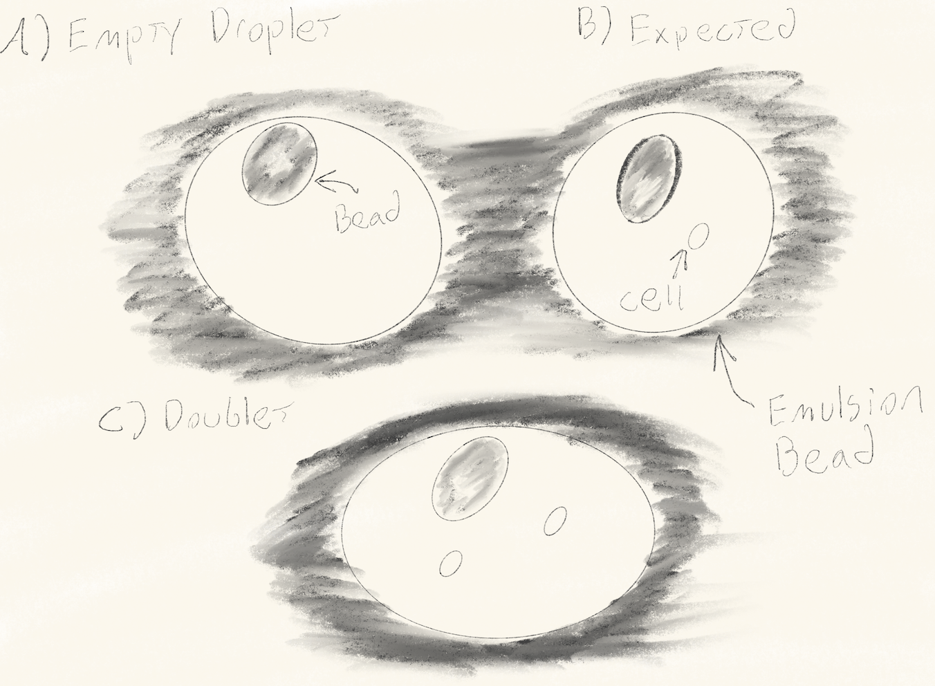
- Empty GEMs contain a bead but no cell -> no transcript capture.
- Doublets contain two cells -> one barcode, mixed transcriptome. Solution: Use QC filters (e.g., total UMI counts) and tools like DoubletFinder. Refer to the figure below for a visual reference
- High Mitochondrial Content
- Elevated MT gene expression suggests the plasma membrane rupture or cell is undergoing apoptosis.
- Rates vary by tissue (Mercer et al. 2011), but >70% is a red flag.
- Ambient RNA Contamination
- If MALAT1 or other housekeeping genes are ubiquitous across clusters, suspect ambient RNA.
- This arises from free-floating RNA (e.g., from lysed cells) being captured in the GEMs. Tool: SoupX can help estimate and subtract ambient signal.
- Flat or Indistinct UMAPs
- If your UMAP looks like a streak or blob, something went wrong.
- Common cause: over-normalization or failure to remove batch effects.
Tools & Resources
- Seurat (R) – Most popular single-cell toolkit
- SingleCellExperiment (R) – More modular S4 framework
- SoupX (R) – Ambient RNA correction
- DoubletFinder (R)- Detect doublet’s in single-cell sequencing data
- rnabio.org: Module 8 – Hands-on single-cell RNA-seq tutorial
- CRI Bioinformatics Workshop - Includes an overview/slides on both single-cell RNA-seq and Spatial Transcriptomics