Rosetta Stone of Data Munging in R

Introduction

In my journey through R, I initially leaned heavily on Base-R, not by choice, but by circumstance. At the time, more advanced data manipulation packages like dplyr from the tidyverse and data.table were either nonexistent or still in their infancy and not yet widely adopted.

This post isn’t meant to spark (or settle) a debate about which syntax is best. Each paradigm, Base-R, tidyverse, and data.table has its own strengths and weaknesses. While I’ll admit a personal preference and deeper knowledge for data.table, I will still reach for the others when a task calls for it.

That said, I do think there are diminishing returns to mastering all three fluently. This guide isn’t about becoming fluent in every flavor of R, it’s about building a practical bridge between them. Whether you’re transitioning from one to another because you need to read a colleagues code or are just trying to understand an answer in stack-overflow, this post aims to serve as a Rosetta Stone of sorts between these dialects.

Where possible I will try and elaborate on how the syntax is working and what it’s doing, however I highly recommend checking out the many detailed guides and tutorials specific to each paradigm of data-munging, I’ve linked a few at the end I think are particularly interesting or easy to follow.

Prepare data

To follow along with the examples presented here you’ll need to install and load the relevant packages. Base-R obviously is already available, tidyverse includes both dplyr and tidyr for data manipulation, and we will need the data.table library as well. We will be using flight data from the nycflights13 package in order to have a standard dataset to manipulate. please refer to the the “Session Info” section of this post for specific package versions.

I also want to note that I would not normally recommend loading both data.table and dplyr libraries in a single R session. Many function names conflict between the two packages. As such you might see me refer explicitly to the function in one package or another with the :: operator. For example both dplyr and data.table have a function first(), in order to explicitly use this function from one package or another we can do data.table::first() or dplyr::first(). This would not be necessary if loading only one library.

# Install packages
install.packages(c('tidyverse', 'data.table', 'nycflights13'))

# load libraries
library(dplyr) # part of tidyverse
library(tidyr) # part of tidyverse
library(data.table)
library(nycflights13) # data to manipulate

Data Structure

Before diving in, it’s helpful to get a basic sense of the data we’ll be working with. Our primary dataset will be flights, which becomes available after loading nycflights13 via library(nycflights13). By default, flights is a tibble, a data structure introduced by the tidyverse. We’ll explore that more in the next section.

For now, what matters is that common base-R functions such as nrow(), ncol(), dim(), summary(), and str() work consistently across data frames, tibbles, and data.table objects—at least for the level of inspection we’ll be doing here. So, don’t worry if you’re not familiar with tibbles yet; these initial exploratory tools behave almost universally.

To begin we will look at the following:

nrow() will give is the number of rows
ncol() will give us the number of columns

dim() will give us both the rows and columns in a two element vector

#######################
### Basic structure ###
nrow(flights) # get number of rows
ncol(flights) # gen number of columns
dim(flights) # get dimensions of object

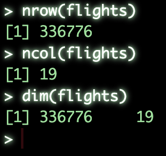
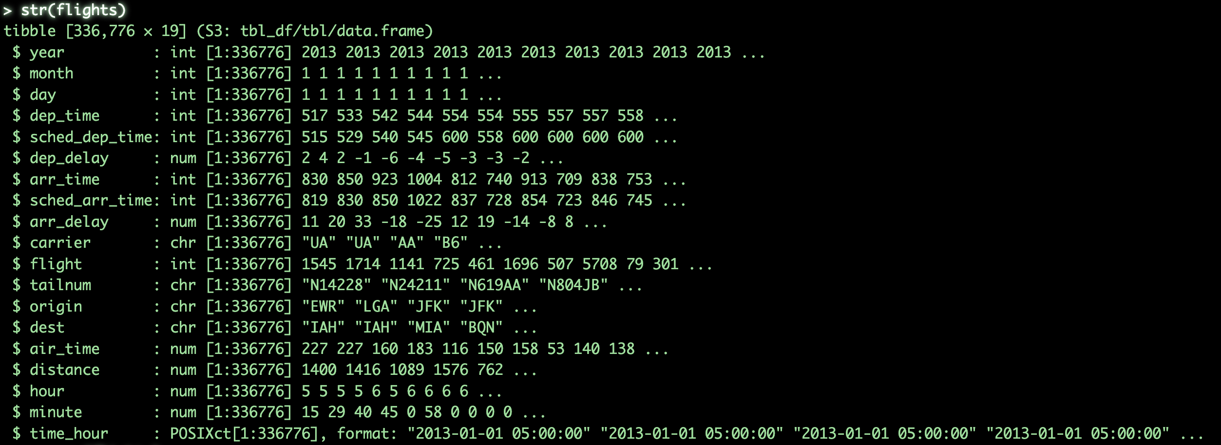
output of structure queries — Output of Basic Structure Commands

str() will output the basic structure of the object which will tell us
- the rows and columns
- columns names
- column class, integer, character, numeric, etc.
- the first few values in the column

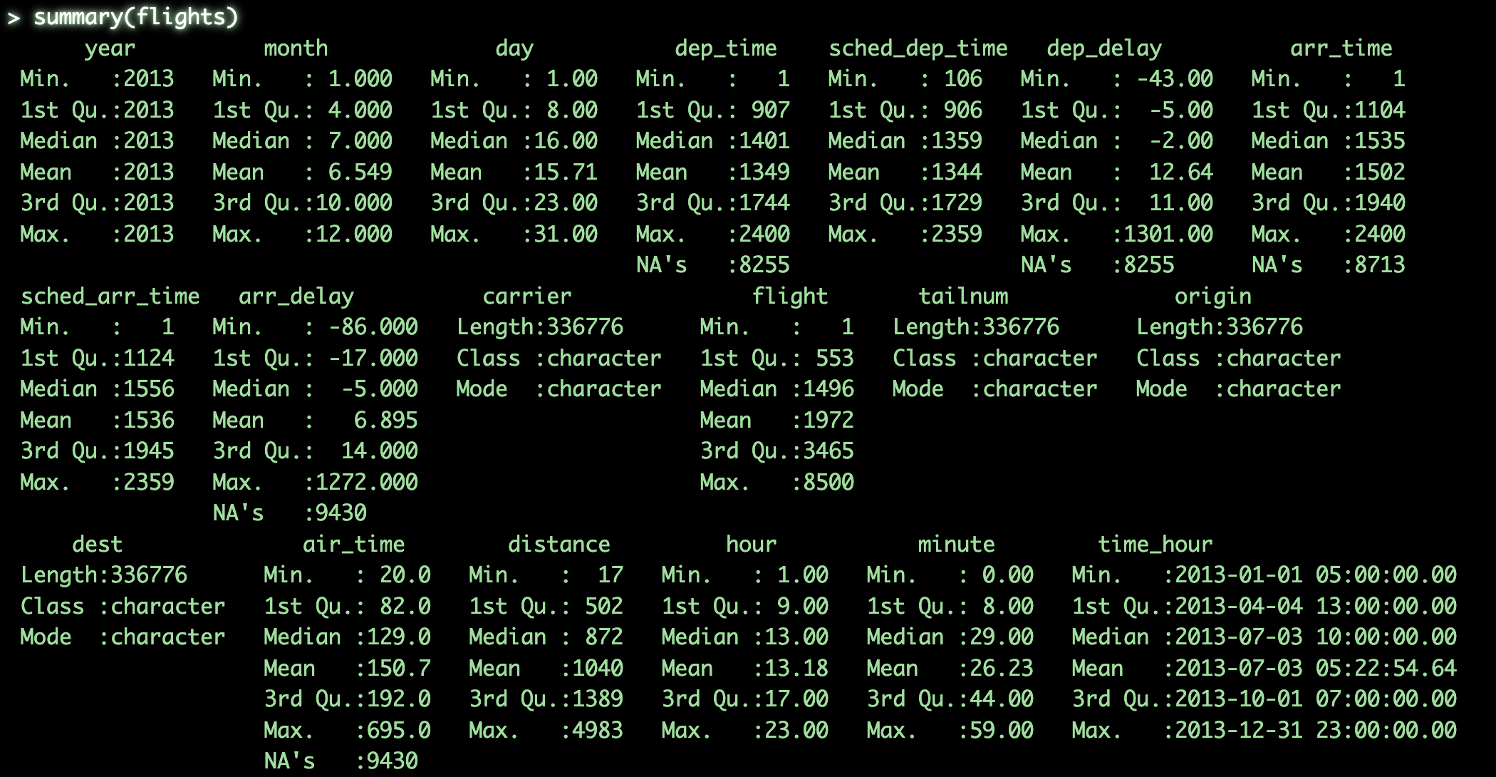
summary() will output basic summary statistics for each column

#######################
# Detailed Structure ##
str(flights) # get structure of object
summary(flights) # get summary statistics for object

output of detailed queries - 1 — Output of str(flights)

output of detailed queries - 2 — Output of summary(flights)

head() will output the first few rows of the object
tail() will output the last few rows of the object
View() will pull up the object in a interactive view-pane, assuming you’re in rstudio

#######################
#### View Object ######
head(flights) # get first few rows
tail(flights) # get last few rows
view(flights) # view object manually 

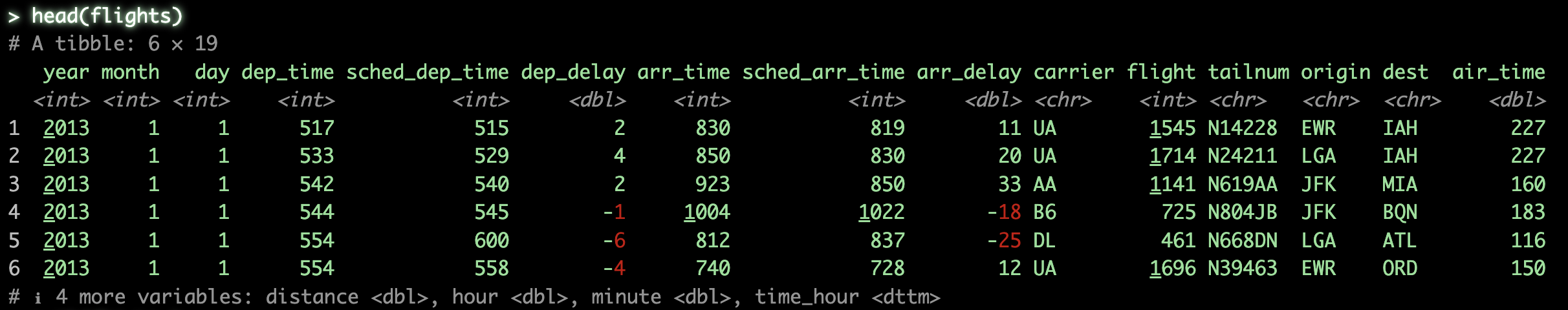
output of view queries - 1 — Output of head(flights)

As we can see, flights contains basic flight information for the year 2013, specifically for New York City airports. The dataset is fairly self-explanatory at a glance, but don’t worry if you’re not familiar with every column. While having a rough idea of the variables can help you understand the logic behind certain operations in later sections, it’s not strictly necessary to follow along.

Formats

Now that we have a basic understanding of the data, it’s time to talk about the formats unique to each paradigm. Most people familiar with R will already recognize the classic data.frame structure, which has been a workhorse in base R for decades. If you’re new to it, don’t worry—it’s essentially a collection of base R vectors (e.g., integer, character, logical) organized into a tabular structure.

In the tidyverse, tibbles are used extensively. These are enhanced data frames designed for better integration with tidyverse functions and more user-friendly behavior. For example, when printing a tibble (like flights, which is already in tibble format), you’ll notice:

Output is limited to the first 10 rows by default
Column types are displayed under each column name
Negative numbers are color-highlighted for readability
The magrittr pipe %>% is used extensively

Tibbles are also technically data.frames under the hood, so nearly all base R functions will work with them as well.

Then there’s data.table, a high-performance extension of data.frame that’s particularly optimized for speed and memory efficiency. Like tibbles, data.tables display column metadata when printed. Unlike tibbles, however, they show the first 5 and last 5 rows by default, which I find especially useful for spotting outliers or missing values early on. One important distinction with data.table is how it handles memory: by default, it modifies objects by reference. That means if you assign a data.table to a new variable, both variables still point to the same underlying data. Any changes to one will affect the other. To create an actual copy, you need to use the copy() function explicitly.

Below, we use the following conversion functions to coerce the same dataset into the formats used by each paradigm:

as.data.frame() -> converts to a base R data frame
as_tibble() -> converts to a tibble (tidyverse)
as.data.table() -> converts to a data.table (data.table package)

# Base-R
flightsDF <- as.data.frame(flights)

# Tidyverse
flightsTB <- as_tibble(flights)

# Data.table
flightsDT <- as.data.table(flights)

Basic Data Manipulation

That’s enough preamble—for now, let’s get into the actual data manipulation. As I mentioned earlier, the goal here isn’t to exhaustively explain every function or syntax nuance within each package. Instead, the following sections will serve as a Rosetta Stone of data munging in R.

Each example is presented in three syntaxes:

Base-R
dplyr (from the tidyverse)
data.table

In most cases, the output across these approaches will be equivalent or near-equivalent.

To keep the focus on practical comparison, I won’t dive into detailed syntax explanations. Instead, I’ll provide general descriptions of what each code block is doing, without going deep into the how.

Selection and Filtering

Select all rows which correspond to Delta airlines (DL)

# Base-R
flightsDF[flightsDF$carrier == 'DL',]

# Tidyverse
flightsTB %>% filter(carrier == 'DL')

# Data.table
flightsDT[carrier == 'DL']

Select the column called “dest”

# Base-R
flightsDF[,'dest']

# Tidyverse
flightsTB %>% select(dest)

# Data.table
flightsDT[,.(dest)]

Select multiple columns by name (origin and dest)

# Base-R
flightsDF[,c('origin', 'dest')]

# Tidyverse
flightsTB %>% select(origin, dest)

# Data.table
flightsDT[,.(origin, dest)]

Select multiple columns by their numeric positions

# Base-R
flightsDF[,c(13,14)]

# Tidyverse
flightsTB %>% select(c(13, 14))

# Data.table
flightsDT[,c(13, 14)]

Column Creation and Deletion

Add a new column called “newCol”, which is the combination of origin and dest

# Base-R
flightsDF$newCol <- paste0(flightsDF$origin, ':', flightsDF$dest)

# Tidyverse
flightsTB <- flightsTB %>% mutate(newCol = paste0(origin, ':', dest))

# Data.table
flightsDT[,newCol := paste0(origin, ':', dest)]

Remove the new column created above

# Base-R
flightsDF$newCol <- NULL

# Tidyverse
flightsTB <- flightsTB %>% select(-c(newCol))

# Data.table
flightsDT[,newCol := NULL]

Basic Data Cleaning

Replace NA values in the “air_time”” column with 0

# Base-R
flightsDF[is.na(flightsDF$air_time),'air_time'] <- 0

# Tidyverse
flightsTB <- flightsTB %>% mutate(air_time = if_else(is.na(air_time), 0, air_time))

# Data.table
flightsDT[is.na(air_time), air_time := 0]

Rename the “dest” column as “destination”

# Base-R
names(flightsDF)[names(flightsDF) == 'dest'] <- 'destination'

# Tidyverse
flightsTB <- flightsTB %>% rename(destination = dest)

# Data.table
setnames(flightsDT, c('dest'), c('destination'))

Sort the object by the longest distance flown in descending order

# Base-R
flightsDF <- flightsDF[order(-flightsDF$distance),]

# Tidyverse
flightsTB <- flightsTB %>% arrange(-distance)

# Data.table
flightsDT <- flightsDT[order(-distance)]

Re-arrange columns so that the column “carrier” comes first

# Base-R
flightsDF <- flightsDF[,c('carrier', names(flightsDF)[names(flightsDF) != 'carrier'])]

# Tidyverse
flightsTB %>% relocate(carrier, .before=year)

# Data.table
setcolorder(flightsDT, 'carrier', before='year')

Grouping and Aggregating

Determine the number of flights from each New York airport

# Base-R
aggregate(flightsDF$origin, by=list(flightsDF$origin), FUN=length) 

# Tidyverse
flightsTB %>% group_by(origin) %>% summarise(count=n())

# Data.table
flightsDT[,.N, by=.(origin)]

Determine the most frequent route flown

# Base-R
aggregate(flightsDF[,c('origin', 'destination')], by=list(flightsDF$origin, flightsDF$destination), FUN=length) |> (\(df) df[order(-df$origin),])() |> (\(df) df[1,])()

# Tidyverse
flightsTB %>% group_by(origin, destination) %>% summarise(count=n()) %>% ungroup() %>% arrange(-count) %>% slice_head(n=1)

# Data.table
flightsDT[,.N,by=.(origin, destination)][order(-N)][1]

Determine the average air-time for the most frequent route for each carrier

# Base-R
aggregate(air_time~carrier,
          data = flightsDF[flightsDF$origin == 'JFK' & flightsDF$destination == 'LAX', ],
          FUN = function(x) c(mean = mean(x, na.rm = TRUE)))
          
# Tidyverse
flightsTB %>% filter(origin == 'JFK' & destination == 'LAX') %>% group_by(carrier) %>% summarise(avg=mean(air_time))

# Data.table
flightsDT[origin == 'JFK' & destination == 'LAX', mean(air_time), by=.(carrier)]

Determine both the average and median air-time for the most frequent route for each carrier

# Base-R
aggregate(air_time~carrier,
          data = flightsDF[flightsDF$origin == 'JFK' & flightsDF$destination == 'LAX', ],
          FUN = function(x) c(mean = mean(x, na.rm = TRUE), median = median(x, na.rm = TRUE)))

# Tidyverse
flightsTB %>% filter(origin == 'JFK' & destination == 'LAX') %>% group_by(carrier) %>% summarise(avg=mean(air_time), med=median(air_time))

# Data.table
flightsDT[origin == 'JFK' & destination == 'LAX', .(avg=mean(air_time), med=median(air_time)), by=.(carrier)]

Reshaping

In this section, we’ll identify the most accurate airline—measured by average departure delay—for each month. We’ll approach this in a slightly roundabout way to demonstrate how data is converted between wide and long formats across each paradigm. The steps for each approach are as follows:

Compute the average flight delay for each month and carrier using the “dep_delay” column
Convert the data into a “wide” format where each month in a column and each row is a carrier
Select only Q1 (Jan. - April) months and convert back to a “long format”

# Base-R
depatureDeviationDF <- aggregate(dep_delay~carrier + month,
                                 data=flightsDF,
                                 FUN=function(x) c(avgDelay = mean(x, na.rm = TRUE)))

depatureDeviationDF_wide <- reshape(depatureDeviationDF,
                                    timevar = "month",
                                    idvar = "carrier",
                                    direction = "wide")
colnames(depatureDeviationDF_wide) <- gsub('dep_delay.', '', colnames(depatureDeviationDF_wide))

depatureDeviationDF_long <- reshape(depatureDeviationDF_wide, 
                                    direction = "long", 
                                    varying = 2:5, 
                                    v.names = "avgDelay", 
                                    timevar = "month", 
                                    times = names(depatureDeviationDF_wide)[2:5], 
                                    idvar = "carrier")
depatureDeviationDF_long <- depatureDeviationDF_long[,c('carrier', 'month', 'avgDelay')]

# Tidyverse
depatureDeviationTB <- flightsTB %>% group_by(month, carrier) %>% summarise(avgDelay=mean(dep_delay, na.rm=TRUE))
departureDeviationTB_wide <- depatureDeviationTB %>% 
  select(carrier, month, avgDelay) %>%
  pivot_wider(names_from = month, values_from = avgDelay)

departureDeviationTB_long <- departureDeviationTB_wide %>%
  pivot_longer(
    cols = 2:5,
    names_to = "month",
    values_to = "avgDelay"
  ) %>%
  select(carrier, month, avgDelay)
  

# Data.table
departureDeviationDT <- flightsDT[,.(avgDelay=mean(dep_delay, na.rm=TRUE)),by=.(month, carrier)]
departureDeviationDT_wide <- dcast(departureDeviationDT, carrier~month, value.var='avgDelay')
departureDeviationDT_long <- melt(departureDeviationDT_wide, id.vars=c('carrier'), measure.vars=c(2:5), variable.name='month', value.name='avgDelay')

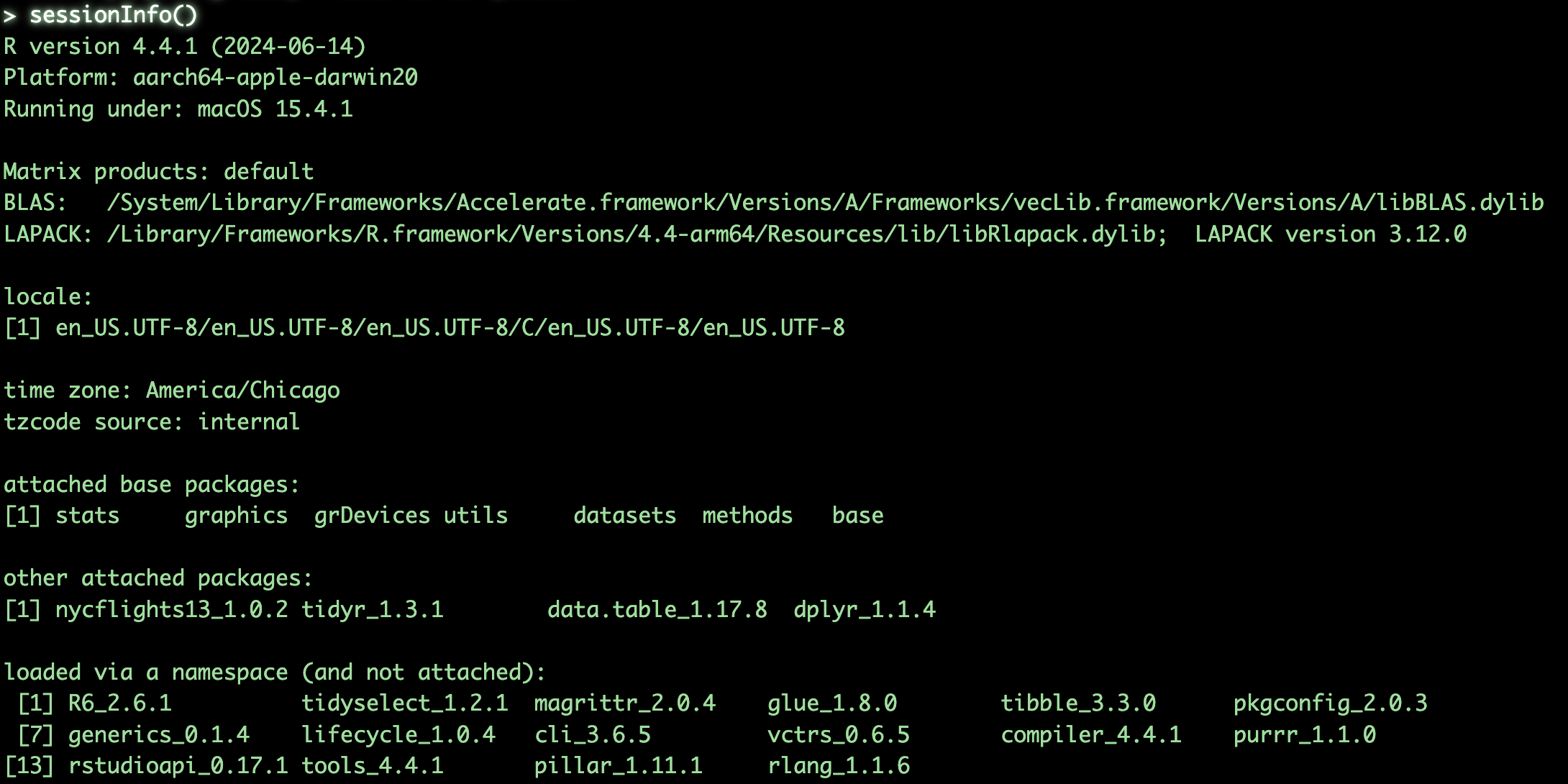
Session Info

This guide was develped on R version 4.4.1, please find specific package versions

Additional Resources

Quick guide to data.table with more in-depth information
tidyr cheat sheet
dplyr cheat sheet
R Code for this post